The three random functions at a glance
Every random formula in Excel is built from one of these. All three work in Excel for Microsoft 365, Excel for the web and Excel on Mac; the version column tells you what older desktop editions support.
| Function | What it returns | Available in |
|---|---|---|
| RAND() | One decimal number from 0 up to, but never exactly, 1. | Every version |
| RANDBETWEEN(bottom, top) | One whole number between bottom and top, both included. | Excel 2007 and later |
| RANDARRAY(rows, columns, min, max, whole) | A whole block of random numbers, decimals or integers, that spills into neighboring cells. | Microsoft 365, Excel 2021 and later |
One thing they share: they are volatile. Every time anything in the workbook changes, or you press F9, Excel recalculates them and you get new numbers. That is perfect for simulations and annoying for raffles, so there is a section below on how to lock results in place.
RANDBETWEEN: a random whole number in a range
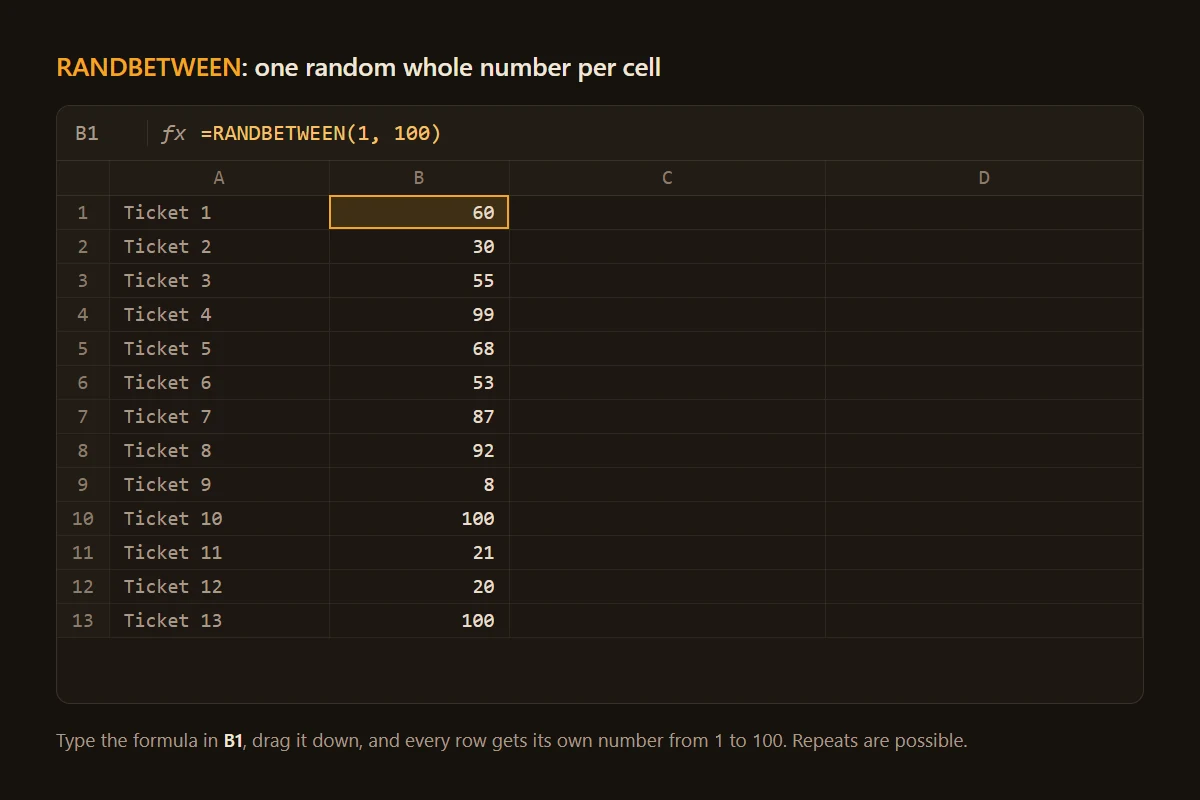
For most people this is the only function they need. Type =RANDBETWEEN(1, 100) into a cell and you get a whole number from 1 to 100. Both ends are included, so 1 and 100 can both come up. Drag the fill handle down and every cell gets its own independent number.
=RANDBETWEEN(1, 6)rolls a die.=RANDBETWEEN(1000, 9999)makes a four-digit code, for example a PIN for a test account.=RANDBETWEEN(-10, 10)works with negative numbers too.=RANDBETWEEN(A1, B1)takes the range from other cells, so you can change the limits without editing the formula.
RANDBETWEEN only returns integers. If you pass it decimals, like =RANDBETWEEN(1.5, 3.5), Excel quietly rounds the limits and you get 2 or 3. For decimal results, use RAND instead.
RAND: random decimals and custom ranges
=RAND() takes no arguments and returns a number like 0.4719276. On its own that is rarely what you want, but a little arithmetic turns it into any range:
| Formula | Result |
|---|---|
| =RAND()*100 | A decimal from 0 to just under 100. |
| =RAND()*(10-5)+5 | A decimal between 5 and 10. The pattern is RAND()*(max-min)+min. |
| =ROUND(RAND()*(10-5)+5, 2) | The same, rounded to two decimal places, for prices or measurements. |
| =NORM.INV(RAND(), 50, 10) | A bell-curve value around 50 with a standard deviation of 10, useful for realistic test scores. |
RAND is also the trick behind shuffling in older versions of Excel. A column of RAND values gives every row a random sort key, which is exactly what you need for the methods further down.
RANDARRAY: many random numbers at once
In Microsoft 365 and Excel 2021, one formula can fill a whole range. The syntax is =RANDARRAY(rows, columns, min, max, whole_number), and every argument is optional.
=RANDARRAY(10)gives ten decimals between 0 and 1 in a column.=RANDARRAY(10, 1, 1, 100, TRUE)gives ten whole numbers from 1 to 100.=RANDARRAY(5, 5, 1, 75, TRUE)fills a 5 by 5 grid, the starting point of a bingo card.=RANDARRAY(20, 1, 0, 1)gives twenty decimals, the same as twenty RAND cells.
The result spills: you type the formula in one cell and Excel fills the cells below and to the right. If something is already in the way you will see a #SPILL! error, so clear the space first. Like RANDBETWEEN, RANDARRAY can repeat values; it is just faster to write.
Random numbers without repeats
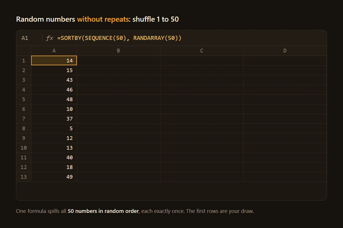
This is the question behind most searches. Ten RANDBETWEEN cells from 1 to 50 will contain a duplicate surprisingly often, about six times out of ten, which is the same math as the birthday paradox. The fix is to stop drawing numbers and start shuffling them: create the full list of numbers once, put it in random order and take as many as you need from the top.

In Microsoft 365 or Excel 2021 and later, one formula does the whole job:
=SORTBY(SEQUENCE(50), RANDARRAY(50))lists the numbers 1 to 50 in random order, each exactly once.=INDEX(SORTBY(SEQUENCE(50), RANDARRAY(50)), SEQUENCE(6))keeps the first six, so you get six different numbers from 1 to 50, like a lottery draw.=TAKE(SORTBY(SEQUENCE(50), RANDARRAY(50)), 6)does the same and is easier to read, but TAKE needs Microsoft 365 or Excel 2024.
In Excel 2019 and older, use two helper columns. Put the numbers 1 to 50 in column A. In B2 enter =RAND() and fill it down. In C2 enter =RANK(B2, $B$2:$B$51) and fill it down. Column C now holds every number from 1 to 50 in random order with no repeats, because two RAND values are practically never equal. Take the first rows of column C for your draw.
If you need several unique draws, a range that changes every day, or numbers you want to exclude, it is easier to let a tool do it. Turn on No repeats in our Random Number Generator, set the number of sets, and download the result as a CSV that opens straight in Excel.
How to randomize a list in Excel
Shuffling a list of names, questions or tasks uses the same idea as above. Suppose your list is in A2:A21.

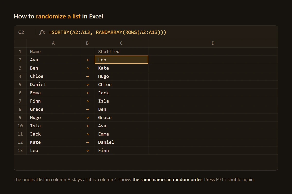
- Microsoft 365 and Excel 2021: in an empty column type
=SORTBY(A2:A21, RANDARRAY(ROWS(A2:A21))). The shuffled list spills down next to the original, which stays untouched. - Any version: in B2 type
=RAND()and fill it down to B21. Select A2:B21, go to Data → Sort, and sort by column B. The list is now in random order, and you can delete column B. - Shuffle again: press F9 to recalculate the formula, or repeat the sort with fresh RAND values.
For a one-off shuffle of a short list it can be faster to skip Excel entirely: paste the lines into our Word Shuffler, choose to shuffle lines, and copy the result back into your sheet.
How to pick a random name or item from a list
To choose one winner from names in A2:A100, combine INDEX with RANDBETWEEN:
=INDEX(A2:A100, RANDBETWEEN(1, ROWS(A2:A100)))picks one cell from the range.=INDEX(A2:A100, RANDBETWEEN(1, COUNTA(A2:A100)))does the same but ignores empty rows at the bottom, as long as the list has no gaps in the middle.=TAKE(SORTBY(A2:A100, RANDARRAY(ROWS(A2:A100))), 3)picks three different winners at once in Microsoft 365.
For a fair raffle, write the result down or freeze it as described in the next section before anyone touches the workbook. Otherwise the next edit will quietly pick a different winner, and that is hard to explain to the people who were watching.
How to stop random numbers from changing
Because random functions recalculate all the time, you need to turn their results into plain values once you are happy with them. There are three ways.
- Paste as values. Select the cells, copy them with Ctrl+C, then paste them back with Paste Special → Values (Ctrl+Alt+V, then V, then Enter). The formulas are replaced with the numbers they showed.
- Convert one cell. Click into a cell with a random formula, select the formula in the formula bar, press F9 and then Enter. Excel stores the current result instead of the formula.
- Switch to manual calculation. Under Formulas → Calculation Options, pick Manual. Nothing recalculates until you press F9. Remember to switch it back, because this setting affects every formula in the workbook, not just the random ones.
Excel has no built-in way to set a seed, so you cannot make RAND produce the same sequence again later. If you need reproducible numbers, freeze them as values or use the Analysis ToolPak described below.
More useful random formulas
Once you know the basic functions, most other random data is one formula away.
| Formula | What it does |
|---|---|
| =RANDBETWEEN(DATE(2026,1,1), DATE(2026,12,31)) | A random date in 2026. Format the cell as a date, or it shows a serial number. |
| =TIME(RANDBETWEEN(9,16), RANDBETWEEN(0,59), 0) | A random time during office hours, from 9:00 to 16:59. |
| =CHAR(RANDBETWEEN(65, 90)) | A random capital letter from A to Z. |
| =IF(RAND()<0.5, "Heads", "Tails") | A coin flip. |
| =CHOOSE(RANDBETWEEN(1,3), "Rock", "Paper", "Scissors") | A random pick from a short fixed list. |
| =RANDBETWEEN(0,1)=1 | A random TRUE or FALSE. |
Random dates are a common need for test data and schedules. If you need them without building a sheet, our Random Date Generator gives you dates in any range, and the Coin Flip does heads or tails with a proper animation.
Weighted random selection
Sometimes options should not be equally likely: a prize wheel where the small prize comes up 70% of the time, or test data where most orders are small. Put the options in A2:A4 and their weights in B2:B4, for example 70, 25 and 5. In C2 type 0, in C3 type =C2+B2, and fill C3 down to C4. Column C now holds the lower edge of each option's slice.
The formula =LOOKUP(RAND()*SUM(B2:B4), C2:C4, A2:A4) picks an option with exactly those odds. RAND times the total lands somewhere between 0 and 100, and LOOKUP returns the option whose slice contains that point. The weights don't have to add up to 100; any positive numbers work.
The Analysis ToolPak: random numbers that don't change
Excel ships with an add-in that writes random numbers as fixed values and supports a seed. Turn it on under File → Options → Add-ins: choose Excel Add-ins, click Go, and tick Analysis ToolPak. Then open Data → Data Analysis → Random Number Generation.
You choose how many columns and rows to fill and a distribution: Uniform, Normal, Bernoulli, Binomial, Poisson, Patterned or Discrete. Entering a Random Seed gives you the same numbers every time, which is handy for teaching and for anyone who needs to repeat an analysis. The numbers it writes are plain values, so they never change on recalculation.
How random is Excel?
Since Excel 2010, RAND uses the Mersenne Twister algorithm, the same family of generator used by Python, R and many statistics packages. For raffles, games, classroom draws, sampling and simulations it is more than random enough: the numbers are evenly spread and show no pattern you could exploit by hand.
It is not a cryptographic generator, though. Don't use Excel to create passwords, encryption keys or anything an attacker might try to predict. For that, use a tool built on the browser's secure generator, like our Password Generator, or the secrets module covered in our guide to random numbers in Python.
Random numbers in Google Sheets
Google Sheets understands =RAND() and =RANDBETWEEN(low, high) exactly like Excel. Its =RANDARRAY(rows, columns) only returns decimals between 0 and 1, so scale it yourself: =ROUNDUP(RANDARRAY(10, 1) * 100) gives ten whole numbers from 1 to 100.
To shuffle a list in Sheets you don't need a formula at all: select the range and choose Data → Randomize range. For six unique numbers from 1 to 50, use =ARRAY_CONSTRAIN(SORT(SEQUENCE(50), RANDARRAY(50), TRUE), 6, 1). Freezing works the same way as in Excel: copy, then Paste special → Values only.
Frequently asked questions
What is the formula for a random number in Excel?
=RANDBETWEEN(1, 100) for a whole number from 1 to 100, with both ends included. Use =RAND() for a decimal between 0 and 1, and =RANDARRAY(rows, columns, min, max, TRUE) to fill a whole range at once in Microsoft 365 or Excel 2021.How do I generate random numbers in Excel without duplicates?
=INDEX(SORTBY(SEQUENCE(50), RANDARRAY(50)), SEQUENCE(6)) returns six different numbers from 1 to 50. In older versions, put =RAND() next to your numbers and rank or sort by that column.Why do my random numbers keep changing in Excel?
How do I randomize the order of a list in Excel?
=SORTBY(A2:A21, RANDARRAY(ROWS(A2:A21))). In any version, add a helper column with =RAND(), sort the list by that column, and then delete it.How do I pick a random name from a list in Excel?
=INDEX(A2:A100, RANDBETWEEN(1, ROWS(A2:A100))). Freeze the result as a value before you announce it, or the next edit will pick someone else.